Free Online Education: Word & Excel Training - Touch Typing - Math & Language Games

In this website you can learn and self practice all the basics of excel
Choose one of the subjects from above, and a list of relevant videos will appear. It includes many tutorial videos with easy step by step manual instructions.

Free Microsoft Word tutorials, as well as the other subjects, could be found on the left menu.

You will notice that all of the learning materials are freely available online, and the videos are short and very easy to understand, planned especially for beginners. 

Though they were recorded in Excel 2007, they are totaly relevant to the 2010 and 2013 versions as well.

For your convenience, the spreadsheets demonstrated in the videos are available for instant download.
This way you can immediately practice what you have just seen and learned.
Just look for the "Try it yourself" link above the video, click it and choose whether to open the spreadsheet inside your browser, or better download it to your computer and then open with Excel.

Who can benefit from these Excel tutorials?

• School and College students learning an IT course (which usually includes the MS Office 2010 applications) and wish to rehearse at home the materials taught in class.
• Job applicants who are going to be tested on their spreadsheet skills as a part of their job interview.
• People already working with this application, who need help with freshening up their skills from time to time, or are looking for some specific answer to their problem such as how to create charts or to use formulas.

Actually anyone who seeks some quick Excel help can benefit from these short online lessons.

What else is there to find on this website?

Free typing practice - how about improving your keyboarding skills? Do you still type with your index fingers? Then this might be the time to advance one step further: You will find a huge section of typing games, enabling you to practice and improve your typing abilities not with boring passages, but with fun, dynamic and challenging activities.

I've also devoted the last couple of years to thoroughly search and index free learning materials on the web, mainly for elementary school, with a special emphasis on the younger ages (mostly 2nd, 3rd & 4th grades), though middle school materials are also presented. You can therefore find a huge assortment of free online math games, some of which (place value, rounding, skip counting, addition & multiplication) I've programmed by myself.

There are also language arts online activities, including games to practice spelling, many crossword puzzles for kids (originally and unique to this website), and also unique word search puzzles. These activities aim to enhance the child's vocabulary as well as spelling skills.

The learning resources on this website are usually used by teachers to complement the materials taught in class, and by homeschool parents wishing to engage their kids with educational interactive activities.

I hope that you can find benefit from this website, and I hope that I succeed just in a tiny bit to bring my vision of "Free Education For All" into reality.

You can contact me at : www.excel-helps.com

How to correct a #VALUE! error

Applies To:  , excel Excel 2013 , Excel 2010 , Excel 2007 , Excel 2016... for Mac , Excel Starter

The most common reason for the #VALUE! error is that a formula is expecting numbers in a cell, but instead it finds spaces, text, or other characters.

Top solution - Try using functions instead of operators

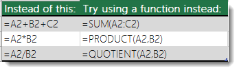
Formulas with math operators like +, -, *, ^ and / may not be able to calculate cells that contain text or spaces. In this case, try using a function instead. Functions will often ignore text values and formulate everything as numbers, eliminating the #VALUE! error.

If you’re not sure what to do at this point or what kind of help you need, you can search for similar questions in the Excel Community Forum, or post one of your own.

If you want to move forward, then the following checklist provides troubleshooting steps to help you figure out what may have gone wrong in your formulas.

Finding where a formula is broken with the Evaluate Formula Wizard

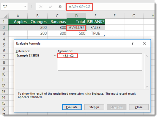
If your formula is throwing a #VALUE! error, but you don't know where it is, you can use the Evaluate Formula Wizard. Select the cell with the error and goto Formulas > Evaluate Formula, and an interactive dialog will appear:

Each time you click the Evaluate button, Excel will step through the formula and calculate each part individually, then display the results. This won't fix your formula, but it can help you figure out where it's breaking, so you can go fix it. In this case the formula =A2+B2+C2 breaks because of a leading space in cell A2, but you can't see it. The Evaluate Formula Wizard does though and it shows that the value is =" "+B2+C2, where the " " indicates a blank space.

Check for hidden spaces inside cells

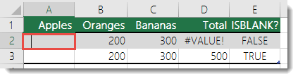
Sometimes cells look blank, when in fact they may have hidden spaces. Double-click a cell that your formula is referencing (or press F2), and check for spaces. In the following illustration, there are extra spaces to the left of cursor in cell A2.

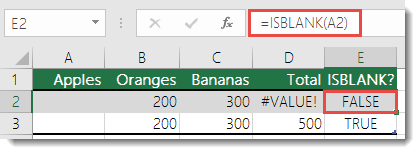
Try deleting the spaces, or select the cell and press Delete to see if the error goes away. If you have many rows to check, you can use the ISBLANK() function in an empty column to see if cells are truly blank or not. In the following illustration, cell A2 has a hidden space that you can’t see, and the ISBLANK function in E2 returns FALSE. Whereas A3 is truly blank and the ISBLANK function returns TRUE.

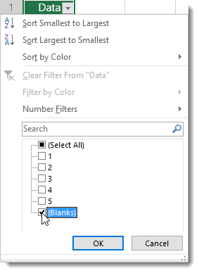
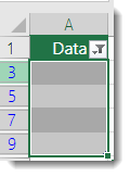
Tip: Use Auto Filter to mass delete blank cells. You can click Data > Filter and Filter for Blanks on the column with blanks (Auto Filter will see cells with leading spaces as blanks as well). Next, select the entire column and press CTRL+G (Goto) > Special > Visible Cells only, then press DELETE to clear everything.

Clean text using the CLEAN function

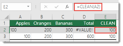
Sometimes when you import data from external sources, it can come into Excel with non-printing characters like ^ or '. Unfortunately, these characters can cause problems in formulas and it can be hard to delete them. However, you can use the CLEAN function to strip the characters out, and convert the values from text to numbers. You can then copy the CLEAN function range and paste just the cell values back over the original range. Here’s how: Select the CLEAN function range, and then press CTRL+C. Select the original cells and click Home > Paste > Paste Special > Values (or Alt > E > S > V for keyboard shortcuts for the PC - For MAC you can use  +OPTION + V > V > Enter).

Clean text using the TRIM function

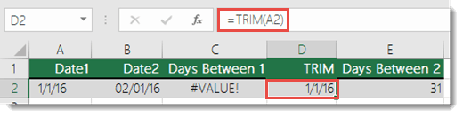
Sometimes leading or trailing spaces can cause problems. Excel will generally try to remove these spaces in simple values. For example, it will remove spaces if you type “ 123”, but it might not be able to do the same with date values like “ 1/1/16”. In this case, you can use the TRIM function to remove those leading and trailing spaces, and then reference the converted TRIM value in your calculation, or use the Copy > Paste Special > Values method to replace the original values.

In this example, leading spaces in the date in A2 cause a #VALUE! error with =B2-A2. But by using =TRIM(A2), we can then use =B2-D2 to resolve the error.

Check if the formula is referencing cells that contain text

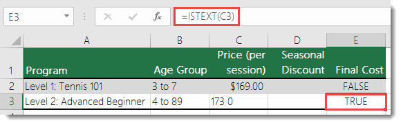
Right-click a cell that the formula is referencing, and then click Format Cells (or use CTRL+1). Make sure the format is not Text. Sometimes this is not practical for more than one cell, so if you have more than one to check, insert a new column and use the ISTEXT() function to see if the cells are formatted as text. In the example below “173 0” isn’t a valid number, so Excel will see it as text. This can often be the result of a typo. Note that ISTEXT won’t resolve the error, it will just tell you if text could be causing the issue.

Your workbook uses a data connection that isn't available

To fix this, restore the data connection, or consider importing the data if possible. This can happen a lot with distributed workbooks, where you might send a workbook to someone who doesn't have the data connection. In cases like this it can be a good idea to create a distribution copy where you copy an entire worksheet(s) and Paste > Special >Values, which will eliminate formulas and links.

Replace the #VALUE! error with something else

Sometimes you just want to replace the #VALUE error with something else like your own text, a zero or a blank cell. In this case you can add the IFERROR() function to your formula. IFERROR() will check to see if there’s an error, and if so, replace it with another value of your choice. If there isn’t an error, your original formula will be calculated. IFERROR will only work in Excel 2007 and later versions. For earlier versions you can use IF(ISERROR()).

Warning: IFERROR is a blanket error handler, meaning that it will suppress all errors, not just the #VALUE! error. It’s not advisable to use IFERROR until you are absolutely certain that your formula performs the way that you want. Otherwise, you won’t see potentially valuable error messages that might indicate you have a problem.

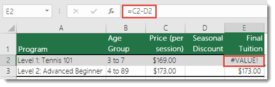
Here’s an example of a formula that has a #VALUE! error due to a leading space in cell D2:

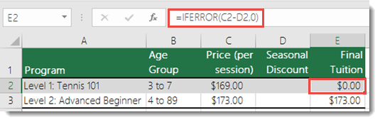
And here’s the same example with IFERROR applied to replace #VALUE! with zero:

You could also use =IFERROR(C2-D2,””) to display nothing instead of 0, or even substitute your own text, like: =IFERROR(C2-D2,”Discount Error”).

Unfortunately, you can see that IFERROR doesn’t actually resolve the error, it simply hides it. So be certain that hiding the error is better than fixing it.

Excel OR Function

Formula examples 

If NOT this or that 

If cell is x or y and z 

If cell is this OR that 

Highlight dates that are weekends

Purpose 

Test multiple conditions with OR

Return value 

TRUE if any arguments evaluate TRUE; FALSE if not.

Syntax 

=OR (logical1, [logical2], ...)

Arguments 

• logical1 - The first condition or logical value to evaluate.
• logical2 - [optional] The second condition or logical value to evaluate.

Usage notes 

Use the OR function to test multiple conditions at the same time, up to 255 conditions total.

For example, to test if the value in A1 OR the value in B1 is greater than 75, use the following formula:

=OR(A1>75,B1<75)

OR can be used to extend the functionality of functions like IF. Using the above example, you can supply OR as the logical_test for an IF function like so:

=IF(OR(A1>75,B1<75), "Pass", "Fail")

This formula will return "Pass" if the value in A1 is greater than 75 OR the value in B1 is greater than 75.

If you enter OR as an array formula, you can test all values in a range against a condition. For example, this array formula will return TRUE if any cell in A1:A100 is greater than 15:

={OR(A1:A100>15}

Notes:

Each logical condition must evaluate to TRUE or FALSE, or be arrays or references that contain logical values.

Text values or empty cells supplied as arguments are ignored.

The OR function will return #VALUE if no logical values are found

Web : excel

How to Use Excel

Excel is a powerful spreadsheet program made by Microsoft Office. You can create and format spreadsheets and workbooks (collections of spreadsheets), build models for analyzing data, write formulas, perform many calculations, and present professional charts. Cash flow statements, income statements, budgets, calendars, or profit and loss statements can all be easily created if you know how to use excel . Open the Excel program. There may be a shortcut on your desktop, or you may need to go to “Start” and then “Programs” to locate the Excel icon. Start a new workbook (an Excel file). Click “File” and “New.” Under “Available templates,” click “Blank Workbook,” then “Create.” A blank workbook will open. Save the workbook. Click the Office button (or File tab if you have an earlier version of Excel) and select “Save as.” Choose a location on your computer to save your file (such as the “my documents” folder), type the name of your workbook in the “File name” box, and be sure your file type is set to “Excel Workbook” Familiarize yourself with the tabs on the ribbon at the top of your workbook.They are File, Home, Insert, Page Layout, Formulas, Data, Review and View. Familiarize yourself with the language needed to use Excel. Knowing the terminology of the technology is important for being able to use it easily and understand step-by-step guides. A row is a section that goes right to left across the screen (indicated by numbers along the left side of the screen). A column is a set of data that goes from the top to the bottom of the worksheet, and it is identified with a letter at the top of the sheet. A cell is any individual square of the worksheet that data may be placed in. 6. Prepare your worksheet for data storage. Every Excel workbook has 3 worksheets by default. Sheet 1 opens by default and you can see this tab at the bottom of the window. Rename a sheet by right clicking on the Sheet 1 tab.  Select “Rename” and type the new name for your sheet. If necessary, add sheets by clicking the button to the right of “Sheet 3” that shows a sheet of paper with a star in the corner. On the top row of your sheet, type a title in each cell to identify what will be placed in each column. For example, you might type Name, Date, and Amount. The rows underneath these titles are for your data. Save frequently. When you are entering data, you may want to save your work frequently by clicking the floppy disk symbol at the top left of your screen or clicking on the office button and selecting “Save.” Alternately, you can hold down the control “Ctrl” key on your keyboard while you type “S.”

Microsoft Excel 2017

Microsoft excel 2017 is the spreadsheet editor included in the popular Microsoft Office suite that will offer you all the essential features when it comes to creating this kind of documents. You'll be able to analyze, manage and share the information to take more precise decisions, with a clear idea of the trends of the most important data for your company

When it comes to spreadsheets, take no chances

It's not every day that you can download a free spreadsheet and be totally satisfied. Microsoft Excel offers total guarantees. Microsoft has spent many years committed to the development of this type of tool, something that translates into an application that works as well as it possibly could.

Features

• Create customized spreadsheets.
• Insert all kinds of statistical tables and graphics to represent the data.
• Import data for the document from an SQL Database or other programs.
• Create calculation rules and customized macros.
• Compare data, detect patterns and trends.
• Recover spreadsheets you had closed accidentally.
• Allows you to work collaboratively.
• Publish the data online and make them accessible wherever you are, where you'll also be able to edit them or access them from your mobile.
• New 'Mini chart" feature to insert small charts into each cell.

Renovated interface to optimize your work

The interface of Microsoft Excel, in accordance with the rest of products of the suite to which it belongs, it includes the 'Ribbon' interface, thus managing to make using the tools easier to use and more accessible. The elements are well distributed, making it more dynamic, which is also encouraged by the new 'Backstage' menu or the integrated visualization of related data and graphics. As well as this, it's worth mentioning the control over styles and icons and the new fillers, that are ideal to provide each value with more visibility.

There are several templates that can be used as a starting point to work, even though you'll have the possibility to customize your own.

Free MS Excel Alternative Software

Are there any free  excel  programs with equivalent features to replace the expensive Microsoft Excel? There are many people everyday who ask this question over the internet, while, the answer is: YES! 

If you are looking for free excel replacement featured with the following functions: 

Formulas and functions 

Auto fill data  , Sorting data  , Data Filter , Pivot Table , Chart Text , Hyperlink,  Freeze Rows and Columns ... , then you will find this free Excel alternative really useful.

Figure 1 Kingsoft Spreadsheets interface

Highly compatible with all Microsoft Excel files. Open *.xls and *.xlsx format files made by Microsoft Excel; create and save spreadsheets in *.xls, *.xlsx.

Figure 2 Open and save Excel format workbooks

Convert Spreadsheets workbooks into PDF files - Export spreadsheet to PDF files directly within the program. Multiple Tabs interface makes it more convenient to switch between several workbooks. It allows you to open many workbooks page on a single window task to optimize your window sequences. 

A great number of formulas are provided for both daily office work and professional business such as Sum, Average, V lookup, Mid, TRIM, TEST, etc. 

Shortcut functions to quickly handle data - These functions include an auto filer, sort ascending, sort descending, auto sum, and more. You can easily edit data by using them.

Count cells that contain text

excel count formula

If you need to count the number of cells that contain text (i.e. not numbers, not errors, not blank), you can do so with the COUNTIF function and a wildcard. In the generic form of the formula (above), rng is a range of cells, and "*" is a wildcard matching any number of characters.

In the example, the active cell contains this formula:

=COUNTIF(B4:B8,"*")

Here's how the formula works:

COUNTIF counts the number of cells that match the supplied criteria. In this case, the criteria is supplied as the wildcard character "*" which matches any number of text characters.

A few notes:

• The logical values TRUE and FALSE are not counted as text
• Numbers are not counted by "*" unless they are entered as text
• A blank cell that begins with an apostrophe (') will be counted.

You can also use SUMPRODUCT to count text values along with the function ISTEXT like so:

=SUMPRODUCT(--ISTEXT(rng))

The double hyphen (called a double unary) coerces the result of ISTEXT from a logical value of TRUE or FALSE, to 1's and 0's. SUMPRODUCT then sums these values together to get a result.

Web : excel